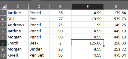
Today, we go over the Freeze Panes feature in excel. A simple but useful tip for working with long spreadsheets. When you work with a long spreadsheet and start scrolling down or to the right, it becomes harder to remember what the data in each cell represents. Take for example the image below.
At first, you’ll have no problem identifying each row or column. You can easily see that the value of cell F8 represents the Unit Cost for a Desk. You can also see that this is related to the Central region. Now, let’s see what happens as you navigate through the spreadsheet.
As we navigate through the spreadsheet, it becomes harder to remember what each cell represents. You may or may not remember that column F represents the Unit Cost. Even if you do, you may forget that this information is for the Central region. Therefore, you may find yourself going up/down or left/right on your spreadsheet to make sense of the data. This process can be very cumbersome depending on how long your spreadsheet is. Here is where the Freeze Panes feature becomes very helpful, so let’s take a quick look at it.
What is the Freeze Panes feature?
The Freeze Panes feature allows you to lock in place a row or column, making them visible always, no matter how much you scroll. There are three variations of this feature.
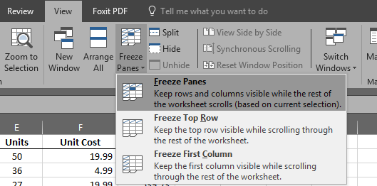
- Freeze Panes – Keep rows and columns visible as you scroll. The number of columns and rows frozen will depend on the current selection. Using our first image as an example, let’s say we want to freeze the top row (headers), but want to always see the region column as well. In this case, you would place the cursor on cell C2 and follow these steps.
- Go to the View menu
- Look for the Freeze Panes feature and select Freeze Panes.
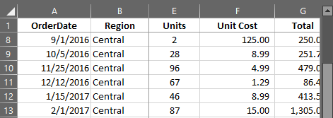
As you see in the image below, no matter how much you scroll down or to the right, you always see the top row and region column.
Note: Always place the cursor on the cell below the row and to the right of the column you want to freeze.
The other two variations are self-explanatory, and you will follow the same steps to activate them. Go to the View Menu > Look for the Freeze Panes feature and pick one of the following options:
- Freeze Top Row – Keep the top row visible while scrolling.
- Freeze First Column – Keep the first column visible while scrolling.
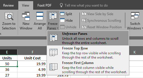
To deactivate any of the Freeze Pane options, all you need to do is:
- Go to the View menu
- Look for the Freeze Panes option and select Unfreeze Panes.


