Using filters in Excel is another way to manage significant amounts of data. On our previous How-To post, we went over the use of the Freeze Panes feature to work with long spreadsheets. Today, we add the use of filters to manage the data better. When you apply filters in excel, you can show only the rows that meet a given criteria while hiding the rest. That way, you can focus on just the data you need at the time.
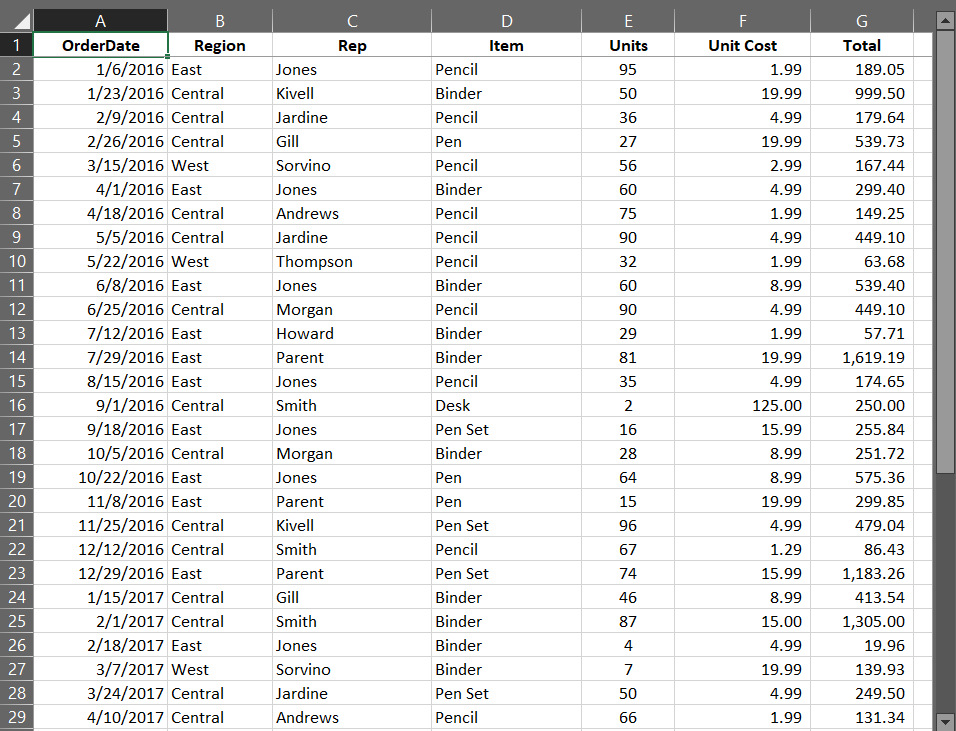
Using our sample spreadsheet, we are going to apply filters to show only those rows where the Region is West.
Activate Filters
To activate the filters feature, follow these steps:
- Place the cursor in one of the cells of your header row. In this case, we use A1.
- Go to the Data menu and click on the Filter button.
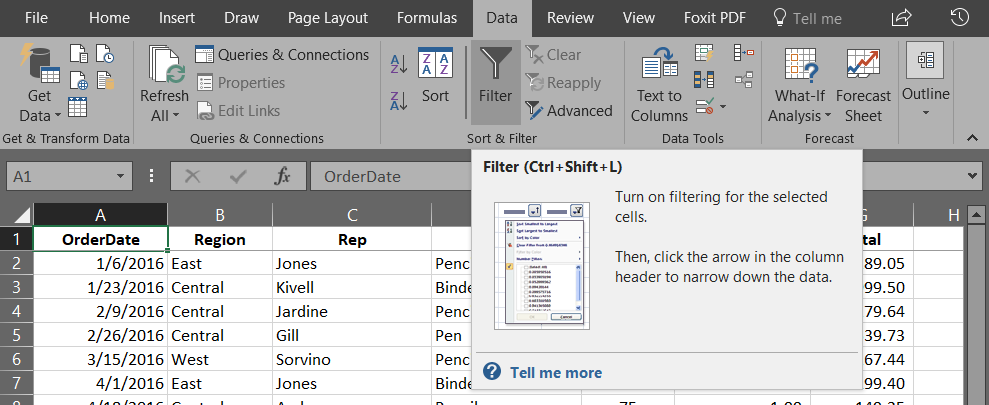
Note: You will notice a drop-down arrow next your column titles.
![]()
Apply Filters
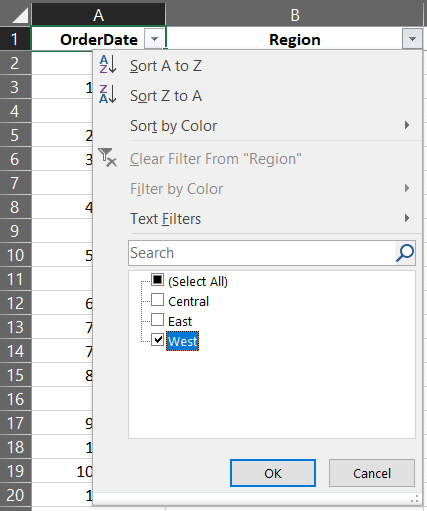
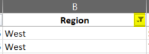
Now that we added the filter feature to our spreadsheet let’s filter the region by doing a click on the drop-down arrow next to the region text and uncheck all the regions except for West.
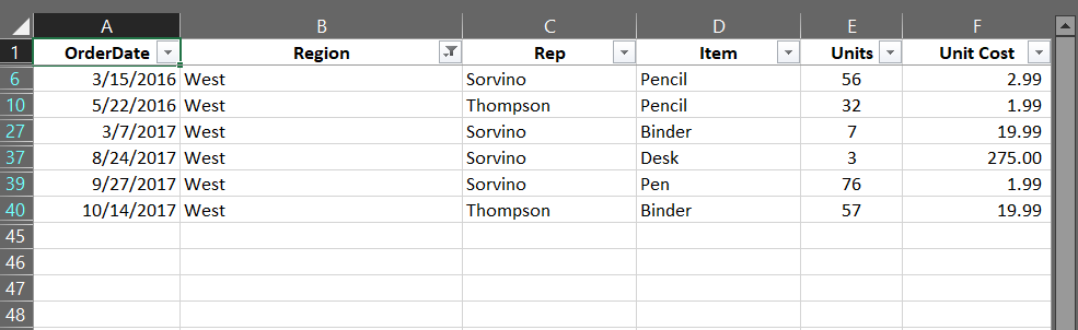
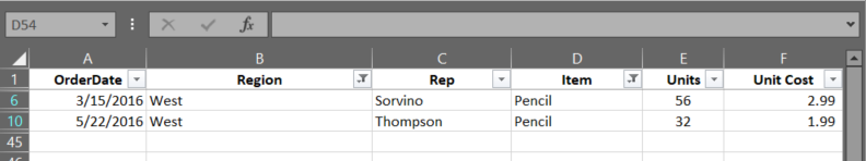
Now, all the rows with a different region are hidden. This allows you to focus on only the data you need. When using the filters feature, you can apply more than one filter to your spreadsheet. Take for example the previous image. In addition to the Region, we are going to apply a filter to the Item column to narrow our search even more.
Note: When you apply a filter to any of the columns, you will see a small filter image next to the text. That way you can tell to which columns you applied a filter.
Clear Filters
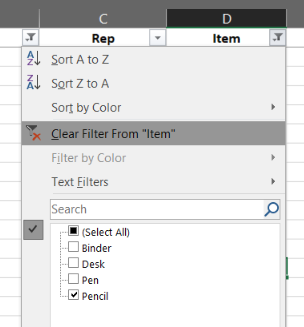
On our previous example, we applied a filter to the Items column. Now, let’s clear the filter by following these steps:
- Click the filter button next to the Item text
- Click the Clear Filter From “Item” option
The spreadsheet will go back to being filtered by Region.